you can also read this article in Medium -> click here
In this article, we will look at object detection using YOLOv12, OpenCV, and Java.
YOLO (You Only Look Once) is one of the most famous object detection systems. It achieves very high speed and accuracy and is one of the easiest ways to get into object detection. The documentation is absolutely perfect, everything is very well explained with lots of examples. It also has a big community of researchers, developers, and enthusiasts who contribute to the project.
I started playing around with YOLO through Python. The integration is so smooth, and I was really impressed by how fast one can start experimenting with object detection. Inference can be done literally in 4 lines:
from ultralytics import YOLO
# Load the YOLOv12 model
model = YOLO("yolo12n.pt")
# Run predictions
results = model.predict('/paht/to/image')
# Display results
results[0].show()
And here is the result:
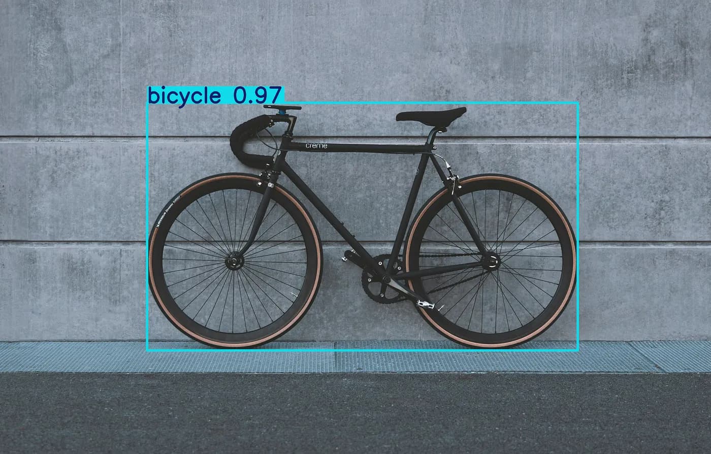
As a Java developer, I also wanted to try this in a simple Java project, but the process there wasn’t that straightforward. Especially understanding the post-processing of the outputs of the inference cost me a lot of time, so I thought it was worth sharing with people who may also struggle with this.
So, in order to start, we need a simple Java Gradle or Maven project and add the OpenCV dependency in build.gradle:
plugins {
    // Apply the application plugin to add support for building a CLI application in Java.
    id 'application'
}

repositories {
    // Use Maven Central for resolving dependencies.
    mavenCentral()
}

dependencies {
    implementation 'org.openpnp:opencv:4.9.0-0'
    ...
Here is also the Maven dependency to add in your pom.xml if you use Maven:
<dependency>
    <groupId>org.openpnp</groupId>
    <artifactId>opencv</artifactId>
    <version>4.9.0-0</version>
</dependency>
Let’s set up some basics next, before moving to the object detection part. I usually start by just reading and showing an image with OpenCV to make sure we got the setup correctly. We’ll load the OpenCV library, then read an image from our resources folder and show it using OpenCV HighGui:
import nu.pattern.OpenCV;
import org.opencv.core.Mat;
import org.opencv.highgui.HighGui;
import org.opencv.imgcodecs.Imgcodecs;

public class ObjectDetectionONLY {
    private static final String IMAGE_NAME = "vase.jpg";

    public static void main(String[] args)
    {
        OpenCV.loadLocally();

        String imagePath = ResourceUtils.getResourcePath(IMAGE_NAME);

        Mat image = Imgcodecs.imread(imagePath);

        HighGui.imshow( "Image", image );
        HighGui.waitKey(0);

        HighGui.destroyAllWindows();
        System.exit(0);
    }
}
I like to prepare some utility classes when working with the file system. It allows me to then focus on the object detection and not think about where to load the images or models from. Here is my ResourceUtils.java helper:
import java.net.URL;

public class ResourceUtils {
    public static String getResourcePath(String resourceName){
        URL resourceUrl = App.class.getClassLoader().getResource( resourceName );
        if(resourceUrl == null){
            throw new RuntimeException("Resource with name "+resourceName+ "not found");
        }
        String resourcePath = resourceUrl.getPath();
        if(resourcePath.isEmpty()) {
            throw new RuntimeException("Error on getting path from resource URL");
        }
        return resourcePath;
    }
}
Alright, now that we have OpenCV in place and we can read and show images, we get to the more interesting part.
We’ll use the OpenCV Deep Neural Network module, which is a perfect starting point for any beginner to get into deep-learning-based computer vision and experiment a bit. Models trained in frameworks like PyTorch or TensorFlow must be converted to the ONNX (Open Neural Network Exchange) format in order to be used directly with the OpenCV DNN module. And that’s what we’re going to do next. Luckily, the conversion of a YOLO Model to .onnx is very simple. You can do it with the YOLO CLI or with Python. We’ll use the YOLOv12 model, which is the latest version available at the time of writing. I recommend using Python through Google Colab for this. Just create a new notebook and add the following code cell:
from ultralytics import YOLO
model = YOLO("yolo12n.pt")
success = model.export(format="onnx")
Run the code from above, and after this, just download the yolo12n.onnx model and save it to your resources folder in the Java project.
YOLO models, including previous versions, are trained on the COCO (Common Objects in Context) dataset by default. This dataset is widely used in the computer vision community for object detection tasks and has 80 classes, including Person, Car, Bicycle, Dog, Cat, and many more.
Let’s add all its classes in the right order to our code:
private static final String[] COCO_CLASSES = {
            "person",
            "bicycle",
            "car",
            "motorcycle",
            "airplane",
            "bus",
            "train",
            "truck",
            "boat",
            "traffic light",
            "fire hydrant",
            "stop sign",
            "parking meter",
            "bench",
            "bird",
            "cat",
            "dog",
            "horse",
            "sheep",
            "cow",
            "elephant",
            "bear",
            "zebra",
            "giraffe",
            "backpack",
            "umbrella",
            "handbag",
            "tie",
            "suitcase",
            "frisbee",
            "skis",
            "snowboard",
            "sports ball",
            "kite",
            "baseball bat",
            "baseball glove",
            "skateboard",
            "surfboard",
            "tennis racket",
            "bottle",
            "wine glass",
            "cup",
            "fork",
            "knife",
            "spoon",
            "bowl",
            "banana",
            "apple",
            "sandwich",
            "orange",
            "broccoli",
            "carrot",
            "hot dog",
            "pizza",
            "donut",
            "cake",
            "chair",
            "couch",
            "potted plant",
            "bed",
            "dining table",
            "toilet",
            "tv",
            "laptop",
            "mouse",
            "remote",
            "keyboard",
            "cell phone",
            "microwave",
            "oven",
            "toaster",
            "sink",
            "refrigerator",
            "book",
            "clock",
            "vase",
            "scissors",
            "teddy bear",
            "hair drier",
            "toothbrush"
    };
Our next steps will be:
- Prepare the input image for the model
- Load the model
- Run the inference
- Extract the bounding boxes from the results
- Visualize the results
We start by preparing the image for the YOLOv12 model. This step includes the resizing (IMG_SIZE is 640px for this YOLO model)
// this step includes swap BGR to RGB
Mat inputBlob = Dnn.blobFromImage(image, 1.0 / 255.0,
                new Size(IMG_SIZE, IMG_SIZE),
                // Here we supply the spatial size that the Convolutional Neural Network expects.
                new Scalar(new double[]{0.0, 0.0, 0.0}),
                true, false);
The last two boolean flags are:
- swapRB: flag which indicates that swapping first and last channels in a 3-channel image is necessary (in OpenCV, the default image format is BGR instead of the more common RGB, that’s why we set this flag to true)
- crop: flag which indicates whether the image will be cropped after resizing or not
The next step is to load our model and set our image blob as an input to the network:
String modelPath = ResourceUtils.getResourcePath(MODEL_NAME);
Net net = Dnn.readNetFromONNX(modelPath);
net.setInput(inputBlob);
Now it’s time to feed the input data through the network and get the output predictions:
Mat outputs = net.forward();After we ran our input image through the network, we got a Mat output object — this is short for “Matrix” and is OpenCV’s primary data structure for storing images or numerical data. These are our Bounding Box Predictions.
Let’s print out the prediction results, which are saved in the outputs :
LOGGER.info("Boxes Output: "+outputs.toString());And let’s concentrate on its dimensions, here the log line:
INFO: Boxes Output: Mat [ 1*84*8400*CV_32FC1, isCont=true, isSubmat=true, nativeObj=0x600003378000, dataAddr=0x15ada8000 ]We see that it has a shape of [1, 84, 8400]. Let’s break it down:
The outputs matrix contains predictions for 8400 potential detections, where each detection has 84 values (4 for bounding box and 80 for class probabilities). The 1 is the batch size, meaning one image is processed.
So, for every one of the 8400 predictions, we have a vector of 84 values that has the following structure:
- 4 values for bounding box coordinates (center_x, center_y, width, height)
- 80 values for class probabilities (80 is the number of classes the model was trained to detect — COCO dataset)
Note: The previous statement only applies for YOLO versions ≥ 8.
YOLO5, for example, has a different output shape:
(batchSize, 25200, 85) (Num classes + box[x,y,w,h] + confidence[c])
It uses anchor boxes, with 3 anchors per grid cell, influencing the number of predictions (25200 = 8400 × 3). We’re not going to get into details here — just wanted to briefly mention it as a side note. If you have any questions, feel free to ask in the comments.
You probably noticed that the boxes output had the structure 1 x 84 x 8400, but we talked about having 8400 predictions, and for each one of them, 84 values. In order to work with this logic properly, we need to transpose the matrix to 8400 x 84. Luckily, this can be done easily with OpenCV in Java:
Mat mat2D = outputs.reshape(1, (int) outputs.size().width); // The second parameter is the number of rows
Core.transpose(mat2D, mat2D);
This will change the structure of our mat2D object to 8400 x 84.
Now we can extract the relevant information from the output. This is going to be our plan:
- Interate over every one of the 8400 rows
- For every row, extract the 80 class probabilities and find the maximum.
- Check this maximum (we can also call this “score”) against a defined threshold (for example, only take predictions that have a score > 0.6)
- Extract the bounding box coordinates
- Draw the bounding box coordinates
var box = new Rect2d();
var className = "";
for (int i = 0; i < mat2D.rows(); i++) {
    List<Double> scores = new ArrayList<>();
    for (int j = 4; j < COCO_CLASSES.length + 4; j++) {
        scores.add(mat2D.get(i, j)[0]);
    }

    MaxScore maxScore = ScoreUtils.findMaxScore(scores);
    if (maxScore.maxValue() < 0.6) {
        continue;
    }

    double width = mat2D.get(i, 2)[0];
    double height = mat2D.get(i, 3)[0];
    double x = mat2D.get(i, 0)[0] - (0.5 * width);
    double y = mat2D.get(i, 1)[0] - (0.5 * height);
    box = new Rect2d(x, y, width, height);
    className = COCO_CLASSES[maxScore.indexOfMax()];
    break;
}
This code snippet seems simple, but it requires an understanding of the underlying structure. Let’s walk through it to really lock it in:
The for-loop iterates through all 8400 prediction rows. For every row, with structure:

The values from index 0 to index 3 are the bounding box predictions.
For our object detection, we first go through the class probabilities (from index 4 to index NUM_CLASSES [80 in our case]) and find the maximum. We call this maxScore — the class with the maximum score is the class of the object that the model found.
The code for ScoreUtils is really just finding the max value from a double array, very simple. We also keep the class index in the MaxScore object:
record MaxScore (double maxValue, int indexOfMax) {}

public class ScoreUtils {

    public static MaxScore findMaxScore(List<Double> array) {
        double max = array.get(0);
        int indexOfMax = 0;
        for (int i = 1; i < array.size(); i++) {
            if (array.get(i) > max) {
                max = array.get(i);
                indexOfMax = i;
            }
        }
        return new MaxScore( max, indexOfMax );
    }
}
After we find the maxScore, we check if it’s above a given threshold, we chose 0.6 here. If that’s not the case, we just move to the next prediction.
If the maxScore is above 0.6, though, we go ahead and extract our bounding box coordinates, save them in the box variable, get the class name of the bounding box prediction, and break the loop.
Now, this is a simplified approach in the spirit of this tutorial. The reason we’re breaking out of the loop here is that we know we only have ONE object to detect in our image. Even if there’s only one object, though, the model usually finds many similar, almost completely overlapping bounding boxes for the same object. Non-Maximum Suppression (NMS) is the standard technique to handle this. NMS keeps only the best detection and removes redundant overlapping boxes.
This step is not too complicated and can be achieved fairly easily with OpenCVs
Dnn.NMSBoxesfunction. Let me know in the comments if you need some help with this.
But, as I said, in order to simplify this, we skip this step — Without NMS (non-maximum suppression) for overlapping boxes, we get very similar bounding box predictions. If we just take one of them, we definitely got a hit (of course, this only works for one object per image).
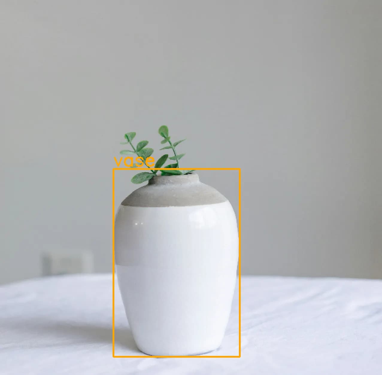
Now we’re already at the easy part — We have a bounding box prediction — let’s just draw it over the image along with the name of the class it belongs to:
Point xy = new Point(box.x, box.y);
Point wh = new Point(box.x + box.width, box.y + box.height);

// In order to draw the boxes correctly, we need to resize the image
Mat resizedImage = new Mat();
Imgproc.resize(image, resizedImage, new Size(IMG_SIZE, IMG_SIZE), Imgproc.INTER_AREA);

Imgproc.rectangle(resizedImage, wh, xy, new Scalar( 0, 165, 255 ), 2);

Point text_point = new Point(box.x, box.y - 5);
Imgproc.putText(resizedImage, className, text_point, Imgproc.FONT_HERSHEY_SIMPLEX, 1, new Scalar( 0, 165, 255 ), 2);

HighGui.imshow( "Image", resizedImage );
HighGui.waitKey(0);

HighGui.destroyAllWindows();
System.exit(0);
I hope you managed to follow along. If you run the program now, you’ll see the result!
(Note: make sure you reference an image you have in your resources folder with one object to be detected — in my case, this was vase.jpg in my IMAGE_NAME constant)
Conclusion
Hopefully, this helped you get a grasp of how to do object detection in Java with the help of OpenCV and YOLOv12. The process is not exactly straightforward, but I hope we managed to tackle all the tricky parts in detail. If you have any questions, I’ll be happy to help!
Thanks for reading!